Libra-RCNN
Pang, Jiangmiao, et al. “Libra r-cnn: Towards balanced learning for object detection.” Proceedings of the IEEE/CVF conference on computer vision and pattern recognition. 2019.
Introduction
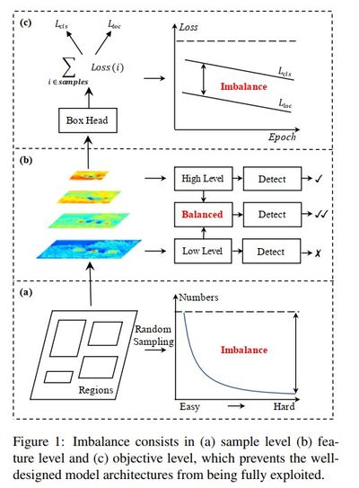
In the object detection community, training pipelines often take a back seat to network architecture and inference optimization. This paper investigates an overlooked aspect of CNN-based detection models: the imbalance phenomenon. The authors decompose this issue into three distinct levels:
- Sample level.
- Feature level.
- Objective level.
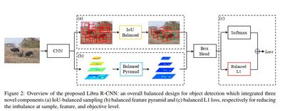
These correspond to the three major components of a detection model: feature extraction, region proposals, and predictors. Building on this categorization, the authors propose the following improvements:
- IoU-balanced sampling.
- Balanced feature pyramid.
- Balanced L1 loss.
So, everything is balanced now.

The authors draw a pretty nice figure to demonstrate their points.
Review and Analysis
Let’s examine each aspect of training imbalance through the lens of this paper.
Sample level Imbalance
Several factors can cause training data to become imbalanced:
-
Data distribution: Bias becomes severe when training data favors certain viewpoints, poses, or object shapes. The model must focus on hard positive samples to generate meaningful gradients and thus learn to generalize. Otherwise, easy samples dominate, driving gradients toward zero. These challenging cases are known as hard positives—not examined in this paper.
-
Data sampling: Two-stage detectors rely on sampling strategies during training. Despite small batch sizes (2 or 4 images) and relatively few ground truth boxes—even with 80 COCO categories, not all images contain many objects—the sampler typically generates thousands of regions. Consequently, easy negative samples overwhelm the training set.
-
Existing solutions: This well-known problem has spawned two noteworthy approaches:
-
OHEM (Online Hard Example Mining): Rather than freezing the network, computing hard negatives, augmenting the training set, and resuming—OHEM directly computes all ROIs in a batch and selects hard negatives on the fly.
-
Focal loss takes a fundamentally different approach by reshaping the standard cross-entropy loss to down-weight well-classified examples. The authors note that Focal Loss shows modest improvement in R-CNN settings. I have only tested it on one-stage models. Interestingly, the YOLOv3 authors also reported limited success with Focal Loss on their architecture.
-
Feature level imbalance
This observation is intriguing when discussing FPN and PANet—region proposal methods employing multi-scale feature mapping:
The methods inspire us that the low-level and high-level information are complementary for object detection. The approach that how they are utilized to integrate the pyramidal representations determines the detection performance. … Our study reveals that the integrated features should possess balanced information from each resolution. But the sequential manner in the aforementioned methods will make integrated feature focus more on adjacent resolution but less on others. The semantic information contained in non-adjacent levels would be diluted once per fusion during the information flow.
Frankly, this section feels underdeveloped. The authors present no experiments to substantiate their claims. Moreover, while they credit inspiration from prior methods, they neglect to explain how these insights led to their proposed approach.
Objective level imbalance
Modern object detection models tackle two tasks simultaneously: label classification and bounding box regression. The difficulty and data distribution of each task can prevent the combined objective from integrating properly. For instance, when box regression dominates, the model achieves strong localization but poor class prediction.
Easy-versus-hard sample imbalance also influences gradient dynamics. When easy samples dominate a batch, gradients become saturated with uninformative signals. Curiously, “easy” does not mean devoid of learning potential. Rather, once the model identifies the “easy” discriminative feature, it tends to ignore other visual cues—essentially fixating on particular positions or features that simplify the task.
In my view, sample and feature imbalance represent the most critical challenges. CNNs can learn diverse viewpoints given adequate training data, but we cannot feasibly capture every object from every conceivable angle. Furthermore, annotation quality varies dramatically with image characteristics. Stock photography and product images yield crisp, accurate bounding boxes; smartphone snapshots and random internet images tell an entirely different story. One glance at COCO annotations confirms this reality.
Proposed Methods
Balanced Feature Pyramid
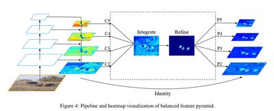
The algorithm for this method is described as the following:
- Rescaling: Resize all feature map into 1 size (intermediate size) using interpolation and max-pooling.
- Integrating: Sum all rescaled feature and normalize it.
- Refining: Directly use convolutions or use non-local module such as Gaussian non-local attention.
- Strengthening: Rescale the obtained feature to the original resolutions.
We can interpret those steps as applying a Pooling layer to form high-level feature, which resembles the final pooling of image retrieval. Hence, it means to improve the abstract level of the feature.
Balanced L1 Loss
The whole formulation of the loss can be seen in the paper. In summary, the authors want to: (1) cap the gradient of the box regression in order to balance with the classification gradient and (2) improve the gradient of the easy samples.
Experiment results
From the result of ablation experiments in Table 2, there are some interesting observations:
- In general, combining 3 methods dramatically improves the average precision of large objects. However, there is not much effect shown in the small objects. In my opinion, small objects still are the most difficult aspect to improve detection models.
- IoU balanced Sampling and Balanced L1 Loss clearly help to improve the Average Precision at IoU=0.75. It means they produce boxes closer to the ground truth.
- The same trend can also be seen on RetinaNet, where the authors used only two methods (Balanced Feature Pyramid and Balanced L1 Loss). Again, the proposed methods improve the overall performance with quite a large margin (+5%), especially on the large objects.
Implementation
In the next two weeks, I will implement the balanced feature pyramid and the balanced L1 loss. I am not sure if I have time for IoU sampler since my focus is on RetinaNet which naturally does not use sampler (but we can trick it a bit and utilize the component). Even though the authors have already released source code using Pytorch, I have to rewrite the whole things through caffe2 and Detectron. It may take a while.
Weighted Component Loss
In a couple of experiments, I have found that there is a big gap between box precision and concept precision. So, my hypothesis is that the box regression loss actually dominates the whole loss of the model. From that, I halve the weight of the box regression and train the model. Here is the results:
| Model | Concept Recall | Concept Precision |
|---|---|---|
| resnet36_tiny12_v0800 (baseline, size 256) | 0.4000 | 0.4445 |
| resnet36_tiny15_v0900 | 0.4122 (+3.05%) | 0.4685 (+5.40%) |
| resnet36_tiny14_v0800 (baseline, size 320) | 0.4194 | 0.4651 |
| resnet36_tiny16_v0800 | 0.3906 (-6.8%) | 0.4984 (+7.16) |
tiny12 and tiny15 are basically the same except tiny15 uses smaller loss weight for box regression (0.5 instead of 1.0). The same settings are applied for tiny14 and tiny16, respectively. From the result, we can see by balancing the loss component, even with the naive approach, it indeed helps the overall performance. However, the second setting is difficult to observe the performance gain. I better use the mAP instead.